38 accept labels in formulas excel 2013
How to Print Labels from Excel, Generate Barcodes, Download Now Use the function "Link data sources" by clicking on the icon in the left toolbar and follow the instructions. Select the option "The data is in a file or in the clipboard". Select the file type, in this case an Excel file was used to print the labels. Select "Excel 97-2003". Select the Excel filecontaining the data you want to use. Excel Workbook wouldn't accept cumulated total formula (Eg. =SUM ... Excel Workbook wouldn't accept cumulated total formula (Eg. =SUM ('Musoma Municipal:Butiama District'!D15) from its sheets. Hi, I have been using Excel over 20 years now though I can't say that I know Excel that much. I have recently denied by Excel to make formula that I have been using over four years now, work.
How to only allow certain values input or enter in Excel? - ExtendOffice Firstly, you need to enter the values you allow input in a list of cells. See screenshot: 2. Then select the cells you want to limit only the certain values input, and click Data > Data Validation. See screenshot: 3. Then, in the Data Validation dialog, under Settings tab, select List from the drop down list under Allow section, and click to ...
Accept labels in formulas excel 2013
What Are the Rules for Excel Names? - Contextures Blog There are rules for Excel Names, and here's what Microsoft says is allowed. It seems clear, but a few of the rules aren't as ironclad as they look: The first character of a name must be one of the following characters: letter. underscore (_) backslash (\). Remaining characters in the name can be. letters. numbers. How to Convert a Formula to a Static Value in Excel 2013 - How-To Geek To do this, click in the cell with the formula and select the part of the formula you want to convert to a static value and press F9. NOTE: When selecting part of a formula, be sure that you include the entire operand in your selection. The part of the formula you are converting must be able to be calculated to a static value. Data types used by Excel | Microsoft Learn Registration data type codes. XLL functions are registered using the C API function xlfRegister, which takes as its third argument a string of letters that encode the return and argument types.This string also contains the information that tells Excel whether the function is volatile, is thread-safe (starting in Excel 2007), is macro sheet equivalent, and whether it returns its result by ...
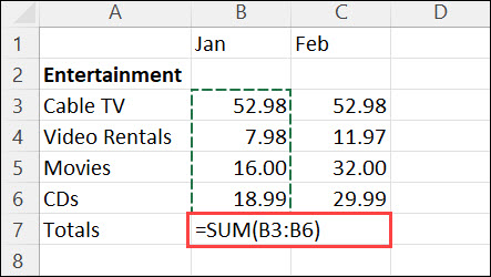
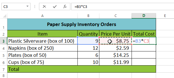
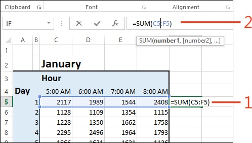
Accept labels in formulas excel 2013. How to mail merge and print labels from Excel - Ablebits.com Sep 26, 2022 · When done, click the OK button.; Step 3. Connect to Excel mailing list. Now, it's time to link the Word mail merge document to your Excel address list. On the Mail Merge pane, choose the Use an existing list option under Select recipients, click Browse… and navigate to the Excel worksheet that you've prepared. Use the Name Manager in Excel - Microsoft Support Create a named range · Be careful about using absolute or relative references in your formula. If you create the reference by clicking on the cell you want to ... [SOLVED] "accept labels in formulas" - Excel Help Forum 4 Apr 2006 — For a new thread (1st post), scroll to Manage Attachments, otherwise scroll down to GO ADVANCED, click, and then scroll down to MANAGE ... Excel- Labels, Values, and Formulas - WebJunction Simple Formula: Click the cell in which you want the answer (result of the formula) to appear. Press Enter once you have typed the formula. All formulas start with an = sign. Refer to the cell address instead of the value in the cell e.g. =A2+C2 instead of 45+57. That way, if a value changes in a cell, the answer to the formula changes with it.
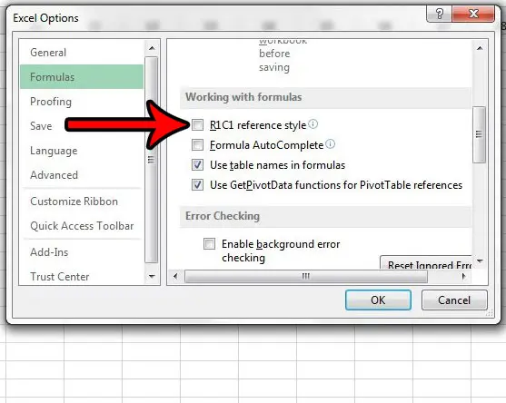
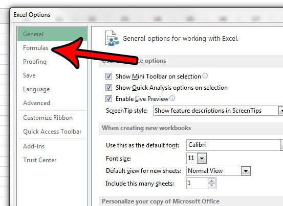
How to use AutoFill in Excel - Ablebits.com Click on File in Excel 2010-2013 or on the Office button in version 2007. Go to Options -> Advanced and untick the checkbox Enable fill handle and cell drag-and-drop . Note. To prevent replacing the current data when you drag the fill handle, make sure that the Alert before overwriting cells check box is ticked. (PDF) Advanced excel tutorial | Adeel Zaidi - Academia.edu Oct 25, 1983 · Individual Data Series In the earlier versions of Excel, you could change the Chart type of an individual data series to a different Chart type by selecting each series at a time. Excel would change the Chart type of the selected data series only. In Excel 2013, Excel will automatically change the Chart type for all data series in the Chart. The Beginner's Guide to Microsoft Excel Online - Zapier May 30, 2017 · Incredibly, the same add-ins designed for Excel 2016 run in Excel Online, so you can use many of the same powerful tools that would otherwise require desktop Excel. To add an add-in to your Microsoft Excel Online spreadsheet, click the Insert menu in Excel Online and select Office Add-ins to browse the store right inside your spreadsheets. Excel 2013, Filter not working for all table content Select the "Table tools" ribbon that is displayed above the other ribbons. Select "Resize table" (at far left of Table tools ribbon). The resize dialog will be displayed. It will be obvious it only rows down to 468 are included in the table by the range shown by default as the current range of the table.
Excel Dashboard Course • My Online Training Hub Power Query gets data from almost any source (a database, the web, Excel, Sharepoint, Salesforce, OData etc), and loads it into Excel or Power Pivot for analysis, report preparation or export. Power Pivot can import millions of rows of data, create relationships between different data sources, and build interactive reports. formatting - How to format Microsoft Excel data labels without trailing ... For a larger dataset, you will need to use a conditional expression to determine all the cell's that have decimal values. One way to do this, is like so: If your numbers are in column B, apply this formula for column C =B1=INT (B1) This will show TRUE if the data is of INT data type (no decimal precision) and FALSE if not. How to Print Labels From Excel - EDUCBA Navigate towards the folder where the excel file is stored in the Select Data Source pop-up window. Select the file in which the labels are stored and click Open. A new pop up box named Confirm Data Source will appear. Click on OK to let the system know that you want to use the data source. Again a pop-up window named Select Table will appear. IFS Function in Excel 2016, 2013, 2010 and 2007 - Office PowerUps Excel 365 or Excel 2019 introduced a new function called IFS. You can add an IFS function in Excel 2016, 2013 or your copy of Excel 2010, or 2007 with the Excel PowerUps add-in. This IFS function in Excel 2016 (or earlier) allows you to specify a series of conditions easily in a single function without having to nest several IF functions.
1. Creating Your First Spreadsheet - Excel 2013: The Missing ...
Stephane M. - Fractional CTO - Unified Remote Work | LinkedIn The fundamental approach of the series was provided in the description of Stat2.1x & appears here again: There will be no mindless memorization of formulas and methods. Throughout the course, the emphasis will be on understanding the reasoning behind the calculations, the assumptions under which they are valid, and the correct interpretation of ...
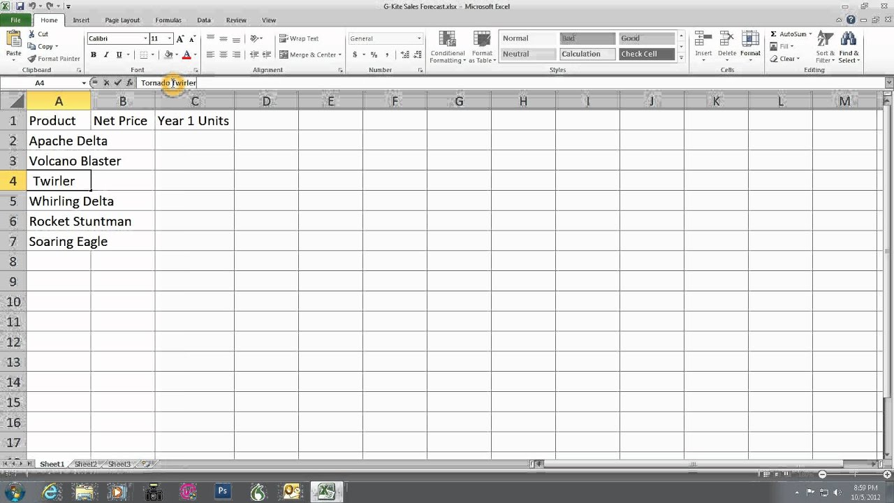
Excel Entering Labels And Values (G)
Excel 2013: Formatting Cells - GCFGlobal.org To use the Bold, Italic, and Underline commands: Select the cell (s) you want to modify. Click the Bold ( B ), Italic ( I ), or Underline ( U) command on the Home tab. In our example, we'll make the selected cells bold. The selected style will be applied to the text.
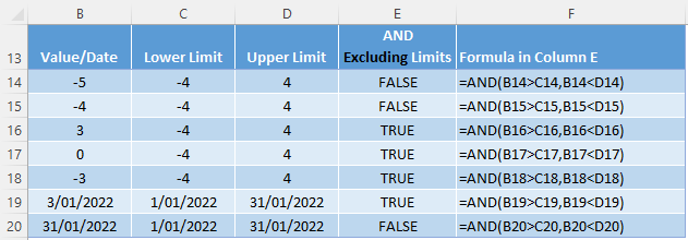
Excel BETWEEN Formula • My Online Training Hub
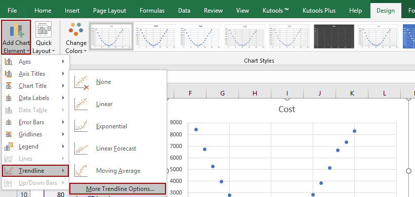
Enable or Disable Excel Data Labels at the click of a button - How To Step 1: Here is the sample data. Select and to go Insert tab > Charts group > Click column charts button > click 2D column chart. This will insert a new chart in the worksheet. Step 2: Having chart selected go to design tab > click add chart element button > hover over data labels > click outside end or whatever you feel fit.
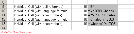
Excel Named Ranges - Natural Language Formulas
AutoFill in Excel - How to Use? (Top 5 Methods with Examples) Fill the range A26:A34 with a series of time values incrementing by one hour. Use the "fill series" option of the AutoFill feature in excel. Step 1: Select cell A25. Step 2: Drag the fill handle till cell A34. Excel has filled the range A26:A34 with the different time values, as shown in the succeeding image.

How to show data labels in PowerPoint and place them ...
Doughnut Chart in Excel | How to Create ... - WallStreetMojo Doughnut Chart is a part of a Pie chart in excel Pie Chart In Excel Making a pie chart in excel can help you with the pictorial representation of your data and simplifies the analysis process. There are multiple kinds of pie chart options available on excel to serve the varying user needs. read more. A pie occupies the entire chart, but it will ...
Excel Ranges: Naming Your Cells in Excel 2019 - dummies
Excel Named Ranges - Natural Language Formulas 1 Sept 2022 — Labels can only be used in formulas that refer to data on the same worksheet; if you want to represent a range on another worksheet then you ...

How to turn on or off automatic calculation of formulas in Microsoft Excel 2013
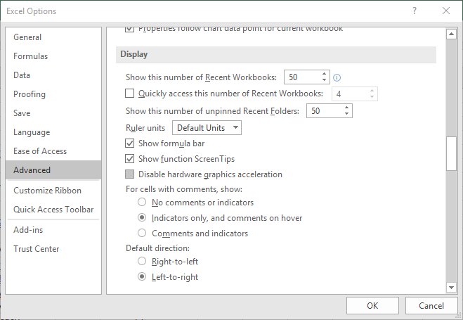
Advanced options - Microsoft Support Discover the meaning of each of Excel's advanced options. ... To be extended, formats and formulas must appear in at least three of the five last rows ...
Controlling Display of the Formula Bar (Microsoft Excel)
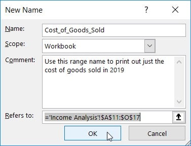
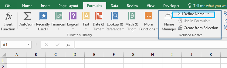
Define and use names in formulas - support.microsoft.com Select Formulas > Create from Selection. In the Create Names from Selection dialog box, designate the location that contains the labels by selecting the Top row, Left column, Bottom row, or Right column check box. Select OK. Excel names the cells based on the labels in the range you designated. Use names in formulas

75+ of the best add-ins, plugins and apps for Microsoft Excel ...
4 steps: How to Create Waterfall Charts in Excel 2013 Select the primary vertical axis (y-axis) and delete as well. Add a chart title -in this case " FY15 Free Cash Flow ". Add data labels by right-clicking one of the series and selecting "Add data labels…". Add labels to each of the series apart from the invisible column. Select the data labels and make them bold, change colour as ...
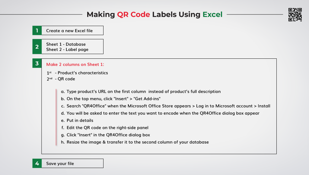
How to Create and Print Barcode Labels From Excel and Word
How to Assign a Name to a Range of Cells in Excel - How-To Geek Select the name you want to insert into the formula by clicking on it in the popup box. The name is inserted into the formula. Press "Enter" to accept the change and update the cell. Note that the result is updated using the exchange rate referred to by the name. Names are very useful if you create complex Excel workbooks with a lot of formulas.

17 Useful Human Resources Formulas and Functions for Excel
Names in formulas - Microsoft Support Select the cell, range of cells, or nonadjacent selections that you want to name. Click the Name box at the left end of the formula bar. Name box Type the name you want to use to refer to your selection. Names can be up to 255 characters in length. Press ENTER. Note: You cannot name a cell while you are changing the contents of the cell.
Displaying Formula Syntax in Excel 2007
Define and use names in formulas - Microsoft Support Select the range you want to name, including the row or column labels. Select Formulas > Create from Selection. In the Create Names from Selection dialog ...
1. Creating Your First Spreadsheet - Excel 2013: The Missing ...
Use defined names to automatically update a chart range - Office Select cells A1:B4. On the Insert tab, click a chart, and then click a chart type. Click the Design tab, click the Select Data in the Data group. Under Legend Entries (Series), click Edit. In the Series values box, type =Sheet1!Sales, and then click OK. Under Horizontal (Category) Axis Labels, click Edit.
Create a simple formula in Excel
How to Lock in Formulas Using $ Sign - Business Insider Aug 2, 2013, 12:08 PM One of the best features in Excel is the ability to plug in a formula and then easily drag it into new cells and have it automatically shift to the corresponding cell values....
:max_bytes(150000):strip_icc()/Capture-5c02fa7ec9e77c00019bc8dc.JPG)
How to Create an Excel Database
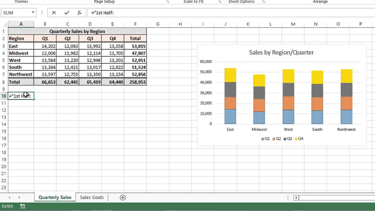
Link a chart title, label, or text box to a worksheet cell In the formula bar, type an equal sign (=). In the worksheet, select the cell that contains the data that you want to display in the title, label, or text box ...
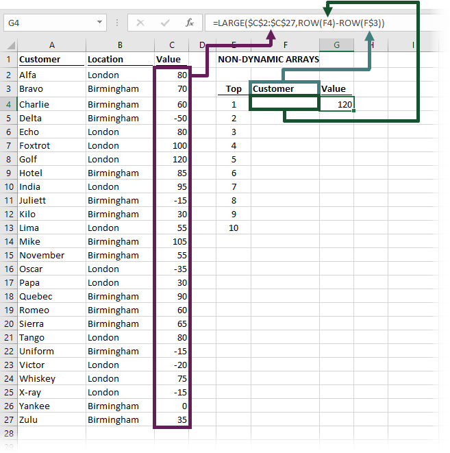
Top 10 with formulas in Excel - Excel Off The Grid
How to Print Labels from Excel - Lifewire Choose Start Mail Merge > Labels . Choose the brand in the Label Vendors box and then choose the product number, which is listed on the label package. You can also select New Label if you want to enter custom label dimensions. Click OK when you are ready to proceed. Connect the Worksheet to the Labels
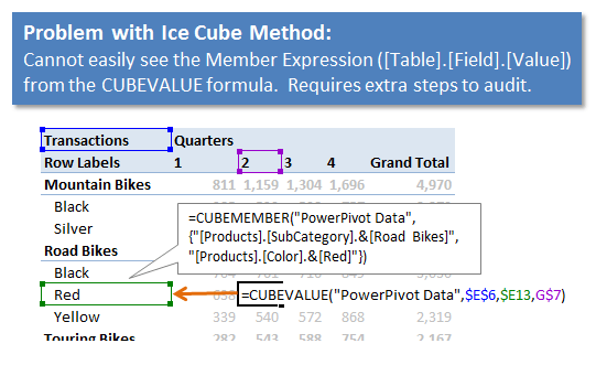
Tips & Tricks for Writing CUBEVALUE Formulas - Excel Campus
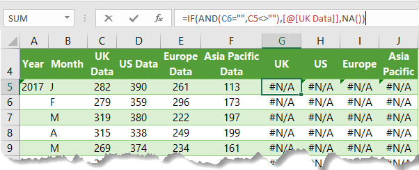
Excel 2013: Label deconfliction in labeled scatter plot Then this formula goes into F2 as an array formula, entered using CTRL + SHIFT + ENTER, and then filled down. =IF (SUM ( (ABS (D2-X)<0.75)* (E2-Y>0)* (E2-Y<0.75))+ (SUM ( (ABS (D2-$D$2:D2)<0.75)* ($E$2:E2=E2))>1),E2,NA ()) This formula creates the series with labels above the point. The formula does two checks:
Help Online - Quick Help - FAQ-112 How do I add a second ...
Adding rich data labels to charts in Excel 2013 | Microsoft 365 Blog To add a data label in a shape, select the data point of interest, then right-click it to pull up the context menu. Click Add Data Label, then click Add Data Callout . The result is that your data label will appear in a graphical callout. In this case, the category Thr for the particular data label is automatically added to the callout too.
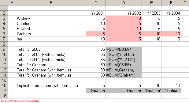
Excel Named Ranges - Natural Language Formulas
How to add data labels from different column in an Excel chart? Right click the data series in the chart, and select Add Data Labels > Add Data Labels from the context menu to add data labels. 2. Click any data label to select all data labels, and then click the specified data label to select it only in the chart. 3.

How To Use LEFT, RIGHT, MID, LEN, FIND And SEARCH Excel Functions
How to make a histogram in Excel 2019, 2016, 2013 and 2010 Sep 29, 2022 · In the Excel Options dialog, click Add-Ins on the left sidebar, select Excel Add-ins in the Manage box, and click the Go button. In the Add-Ins dialog box, check the Analysis ToolPak box, and click OK to close the dialog. If Excel shows a message that the Analysis ToolPak is not currently installed on your computer, click Yes to install it.

How to Use Excel Pivot Table GetPivotData
Repeat All Item Labels In An Excel Pivot Table | MyExcelOnline STEP 1: Click in the Pivot Table and choose PivotTable Tools > Options (Excel 2010) or Design (Excel 2013 & 2016) > Report Layouts > Show in Outline/Tabular Form STEP 2: Now to fill in the empty cells in the Row Labels you need to select PivotTable Tools > Options (Excel 2010) or Design (Excel 2013 & 2016) > Report Layouts > Repeat All Item Labels

How to create an Excel summary table using UNIQUE and SUMIFS
Array formulas and functions in Excel - examples and guidelines An array formula does not need an additional column since it perfectly stores intermediate results in memory. So, you just enter the following formula and press Ctrl + Shift + Enter: =MAX (C2:C6-B2:B6) Example 2. A multi-cell array formula in Excel
1. Creating Your First Spreadsheet - Excel 2013: The Missing ...
Excel 2016 - How to Use Formulas and Functions - UniversalClass.com To do this, we are going to click Insert Function on the Ribbon under the Formulas tab. Once again, we enter "average of cells" in the "Search for a Function field," then click the Go button. Select Average, then click OK. Excel prompts us for our arguments. The arguments are the cells or values that we want to use to calculate the function.
How to Display a Label Within a Formula on Excel : MIcrosoft Excel Tips
Data types used by Excel | Microsoft Learn Registration data type codes. XLL functions are registered using the C API function xlfRegister, which takes as its third argument a string of letters that encode the return and argument types.This string also contains the information that tells Excel whether the function is volatile, is thread-safe (starting in Excel 2007), is macro sheet equivalent, and whether it returns its result by ...
How to use Names in Formulas in Excel
How to Convert a Formula to a Static Value in Excel 2013 - How-To Geek To do this, click in the cell with the formula and select the part of the formula you want to convert to a static value and press F9. NOTE: When selecting part of a formula, be sure that you include the entire operand in your selection. The part of the formula you are converting must be able to be calculated to a static value.
Why Are My Column Labels Numbers Instead of Letters in Excel ...
What Are the Rules for Excel Names? - Contextures Blog There are rules for Excel Names, and here's what Microsoft says is allowed. It seems clear, but a few of the rules aren't as ironclad as they look: The first character of a name must be one of the following characters: letter. underscore (_) backslash (\). Remaining characters in the name can be. letters. numbers.

Automatically create "Dimension Counts" in your OData Excel ...
Excel Formulas: Simple Formulas
Why Are My Column Labels Numbers Instead of Letters in Excel ...

Microsoft Excel - Wikipedia
Excel IF AND OR Functions Explained • My Online Training Hub
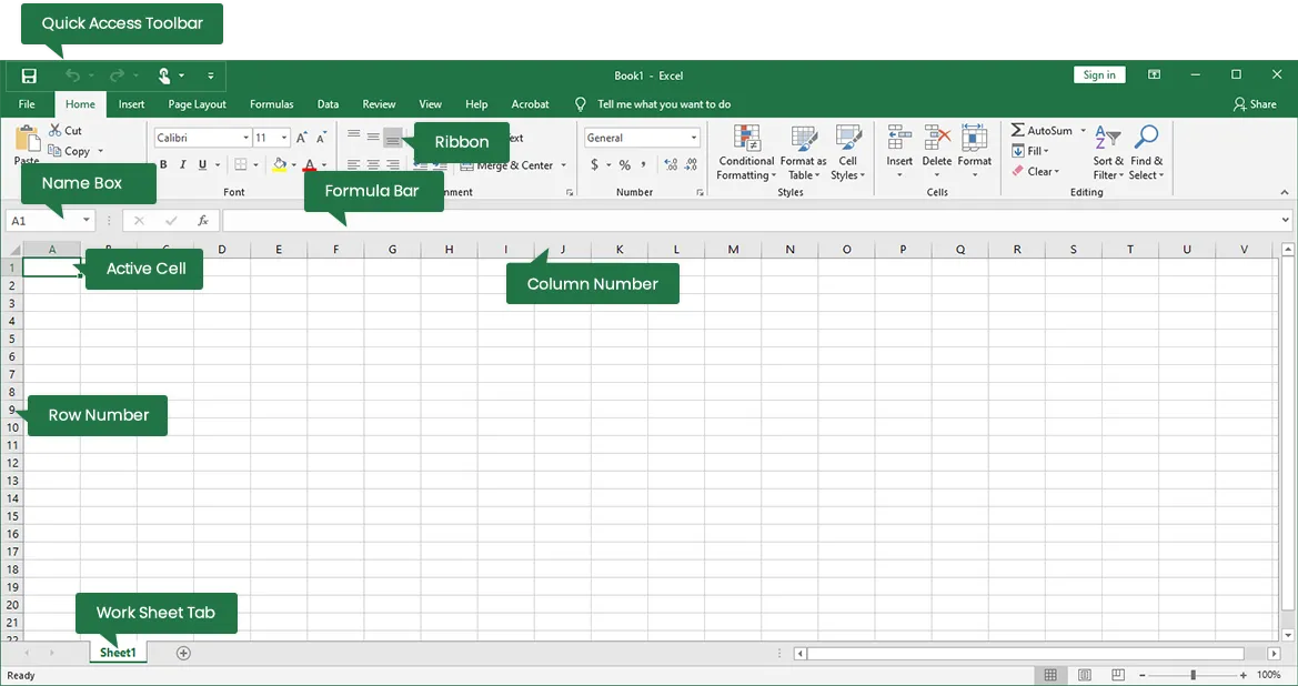
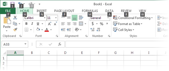
The Excel Interface - Excel Training | Training Connection
Excel Shortcuts to Zoom In and Out in Your Worksheets (4 ...
Dynamically Label Excel Chart Series Lines • My Online ...
Microsoft Excel 2013 – Level 1
Using Formulas and Functions in Microsoft Excel 2013 ...
How to add best fit line/curve and formula in Excel?
1. Creating Your First Spreadsheet - Excel 2013: The Missing ...
Post a Comment for "38 accept labels in formulas excel 2013"