38 excel chart show labels

How to create waterfall chart in Excel 2016, 2013, 2010 - Ablebits.com Jul 25, 2014 · A waterfall chart is also known as an Excel bridge chart since the floating columns make a so-called bridge connecting the endpoints. These charts are quite useful for analytical purposes. If you need to evaluate a company profit or product earnings, make an inventory or sales analysis or just show how the number of your Facebook friends ... Create a Clustered AND Stacked column chart in Excel (easy) In addition, let’s add the additional text box inside the Chart Area that will show a text definition for the secondary Data Labels. To do that, let’s select the Chart Area, then Go To: INSERT tab on the Excel Ribbon > Text Section > Text Box (alternatively: INSERT tab on the Excel Ribbon > Illustrations Section > Text Box)

How to Conditionally Show or Hide Charts - Excel Chart … Nov 05, 2008 · In a complicated Excel 2003 chart, which has two 4-point area chart series to highlight a background range, and an XY series with custom markers (pasted shapes) and more then 4 points, only the first four points appear with their custom markers, though the code that applies the markers does not fail, and the data labels for the marker-less ...

Excel chart show labels

How to Make a Spreadsheet in Excel, Word, and Google Sheets - Smartsheet Jun 13, 2017 · Either insert a Microsoft Excel Chart or a Microsoft Excel Worksheet. Selecting either of these options will open Excel so you can create and edit a fully functional spreadsheet that will then appear as-is in the Word document. ... You can select the Plot Area where the graph is stored, the Chart Area where all the axis labels exist, or any ... How to Show Percentage in Pie Chart in Excel? - GeeksforGeeks Jun 29, 2021 · It can be observed that the pie chart contains the value in the labels but our aim is to show the data labels in terms of percentage. Show percentage in a pie chart: The steps are as follows : Select the pie chart. Right-click on it. A pop-down menu will appear. Click on the Format Data Labels option. The Format Data Labels dialog box will appear. How to Change Excel Chart Data Labels to Custom Values? - Chandoo.org May 05, 2010 · First add data labels to the chart (Layout Ribbon > Data Labels) Define the new data label values in a bunch of cells, like this: Now, click on any data label. This will select “all” data labels. Now click once again. At this point excel will select only one data label.

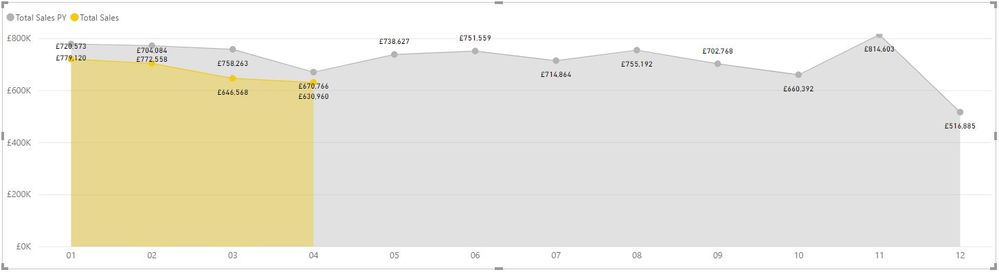
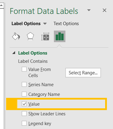
Excel chart show labels. How to Make a Column Chart in Excel: A Guide to Doing it Right Excel offers a 100% stacked column chart. In this chart, each column is the same height making it easier to see the contributions. Using the same range of cells, click Insert > Insert Column or Bar Chart and then 100% Stacked Column. The inserted chart is shown below. A 100% stacked column chart is like having multiple pie charts in a single chart. How to hide zero data labels in chart in Excel? - ExtendOffice If you want to hide zero data labels in chart, please do as follow: 1. Right click at one of the data labels, and select Format Data Labels from the context menu. See screenshot: 2. In the Format Data Labels dialog, Click Number in left pane, then select Custom from the Category list box, and type #"" into the Format Code text box, and click Add button to add it to Type list box. How to Use Cell Values for Excel Chart Labels - How-To Geek Mar 12, 2020 · The column chart will appear. We want to add data labels to show the change in value for each product compared to last month. Select the chart, choose the “Chart Elements” option, click the “Data Labels” arrow, and then “More Options.” Uncheck the “Value” box and check the “Value From Cells” box. Actual vs Budget or Target Chart in Excel - Excel Campus Aug 19, 2013 · Next you will right click on any of the data labels in the Variance series on the chart (the labels that are currently displaying the variance as a number), and select “Format Data Labels” from the menu. On the right side of the screen you should see the Label Options menu and the first option is “Value From Cells”.

How to Change Excel Chart Data Labels to Custom Values? - Chandoo.org May 05, 2010 · First add data labels to the chart (Layout Ribbon > Data Labels) Define the new data label values in a bunch of cells, like this: Now, click on any data label. This will select “all” data labels. Now click once again. At this point excel will select only one data label. How to Show Percentage in Pie Chart in Excel? - GeeksforGeeks Jun 29, 2021 · It can be observed that the pie chart contains the value in the labels but our aim is to show the data labels in terms of percentage. Show percentage in a pie chart: The steps are as follows : Select the pie chart. Right-click on it. A pop-down menu will appear. Click on the Format Data Labels option. The Format Data Labels dialog box will appear. How to Make a Spreadsheet in Excel, Word, and Google Sheets - Smartsheet Jun 13, 2017 · Either insert a Microsoft Excel Chart or a Microsoft Excel Worksheet. Selecting either of these options will open Excel so you can create and edit a fully functional spreadsheet that will then appear as-is in the Word document. ... You can select the Plot Area where the graph is stored, the Chart Area where all the axis labels exist, or any ...

Solved: Area chart data labels not in correct positions ...

Stagger long axis labels and make one label stand out in an ...

How to Get Colors in Excel Chart Data Lables - Formatting Trick

How to Show Percentages in Stacked Column Chart in Excel ...

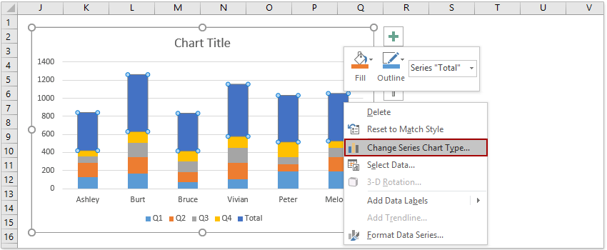
How to add total labels to stacked column chart in Excel?

How to show data labels in PowerPoint and place them ...

Two-Level Axis Labels (Microsoft Excel)

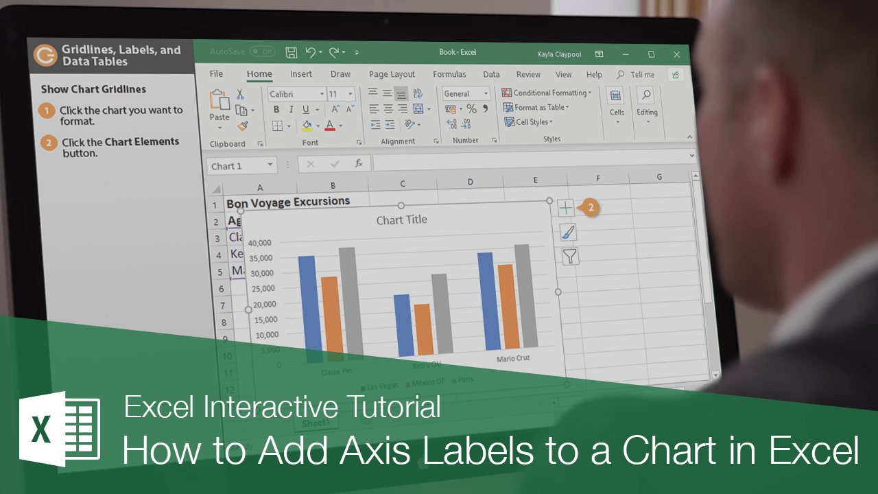
How to Add Axis Labels to a Chart in Excel | CustomGuide

Enable or Disable Excel Data Labels at the click of a button ...

How to add live total labels to graphs and charts in Excel ...

How to Use Cell Values for Excel Chart Labels

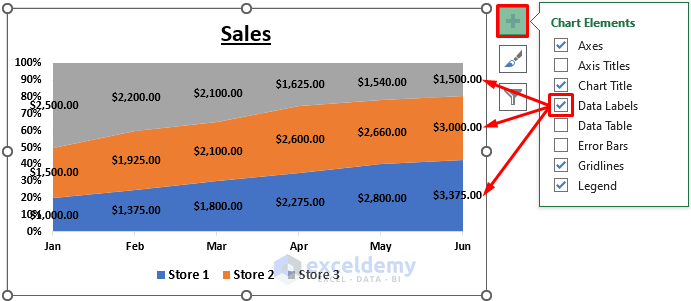
Excel Area Chart Data Label & Position - ExcelDemy

How to Add Data Labels to an Excel 2010 Chart - dummies

How to Customize Your Excel Pivot Chart Data Labels - dummies

How to Use Cell Values for Excel Chart Labels

data visualization - How do you put values over a simple bar ...

microsoft excel - Adding data label only to the last value ...

How to use data labels in a chart

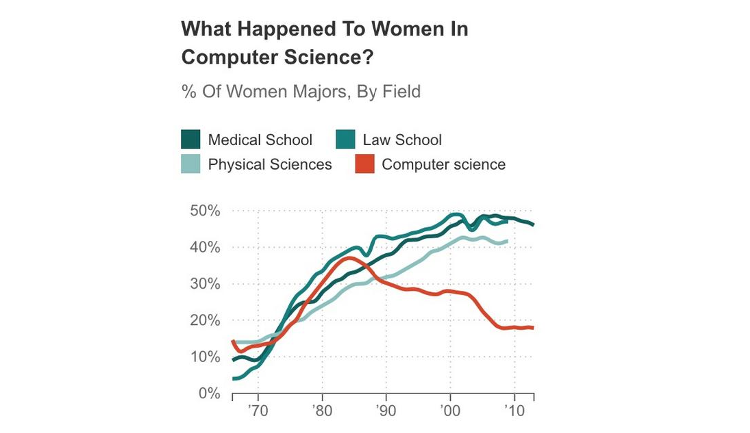
Directly Labeling Your Line Graphs | Depict Data Studio

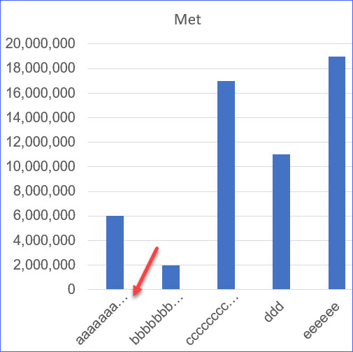
How to Wrap X Axis Labels in an Excel Chart - ExcelNotes

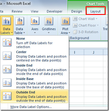
Excel 2010: Show Data Labels In Chart

Add or remove data labels in a chart

Is there a way to add data labels as percentages on the ...

Directly Labeling in Excel

How to add data labels from different column in an Excel chart?

How to Place Labels Directly Through Your Line Graph in ...

How to Change Excel Chart Data Labels to Custom Values?

Add or remove data labels in a chart

Display Customized Data Labels on Charts & Graphs

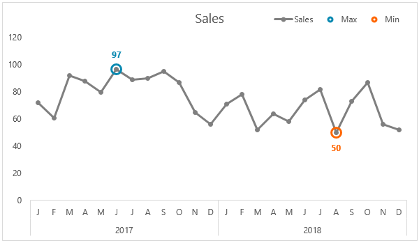
Label Excel Chart Min and Max • My Online Training Hub

Adding rich data labels to charts in Excel 2013 | Microsoft ...

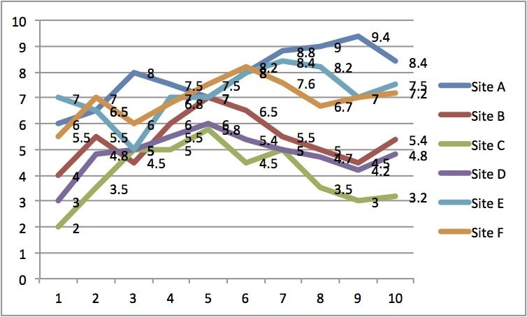
Directly Labeling Excel Charts - PolicyViz

Excel sunburst chart: Some labels missing - Stack Overflow

How to Add Axis Labels to a Chart in Excel | CustomGuide

Adding rich data labels to charts in Excel 2013 | Microsoft ...

Custom Excel Chart Label Positions • My Online Training Hub

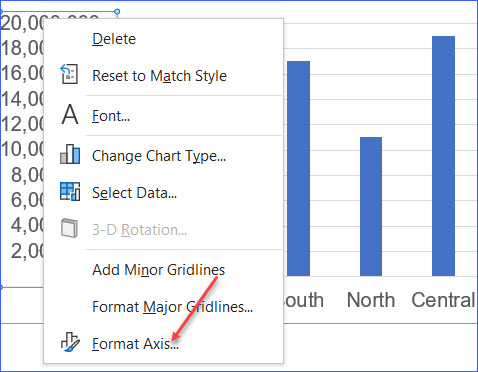
How to Format Axis Labels as Millions - ExcelNotes

Excel charts: add title, customize chart axis, legend and ...

Share :